#4. Logistic Regression with a Neural Network midset

* Overview of the Problem set:

 

- dataset "data.h5" contains:

    1) a training set of m_train images labeled as cat(y=1) or non-cat(y=0)

    2) a test set of m_test images labeled as cat of non-cat

    3) each image is of shape(height=num_px, width=num_px, channel=3) 

 

- training & train data set의 모양을 (num_px*num_px, 3)에서 싱글 벡터(num_px*num_px*3, 1로 만들어준다 

# 행렬 X(a, b, c, d)를 X_flatten(b*c*d, a)로 만들기(X^T)
X_flatten = X.reshape(X.shape[0], -1).T

- Deep Learning에서 common preprocessing step 중 하나는 데이터셋을 center & standardize하는 작업이다. 평균을 전체 numpy array에서 뺀 다음 표준편자로 나누어 주는 작업인데, 이 예시는 간단하므로 255로 나눠주는 것으로 이를 대체함.

 

- summary: pre-processing a new dataset

    1) 모양과 차원을 파악한다.

    2) 데이터이 벡터 형식이 되도록  reshape해준다.

    3) standardize

 

* General Architecture of the learning algorithm

 

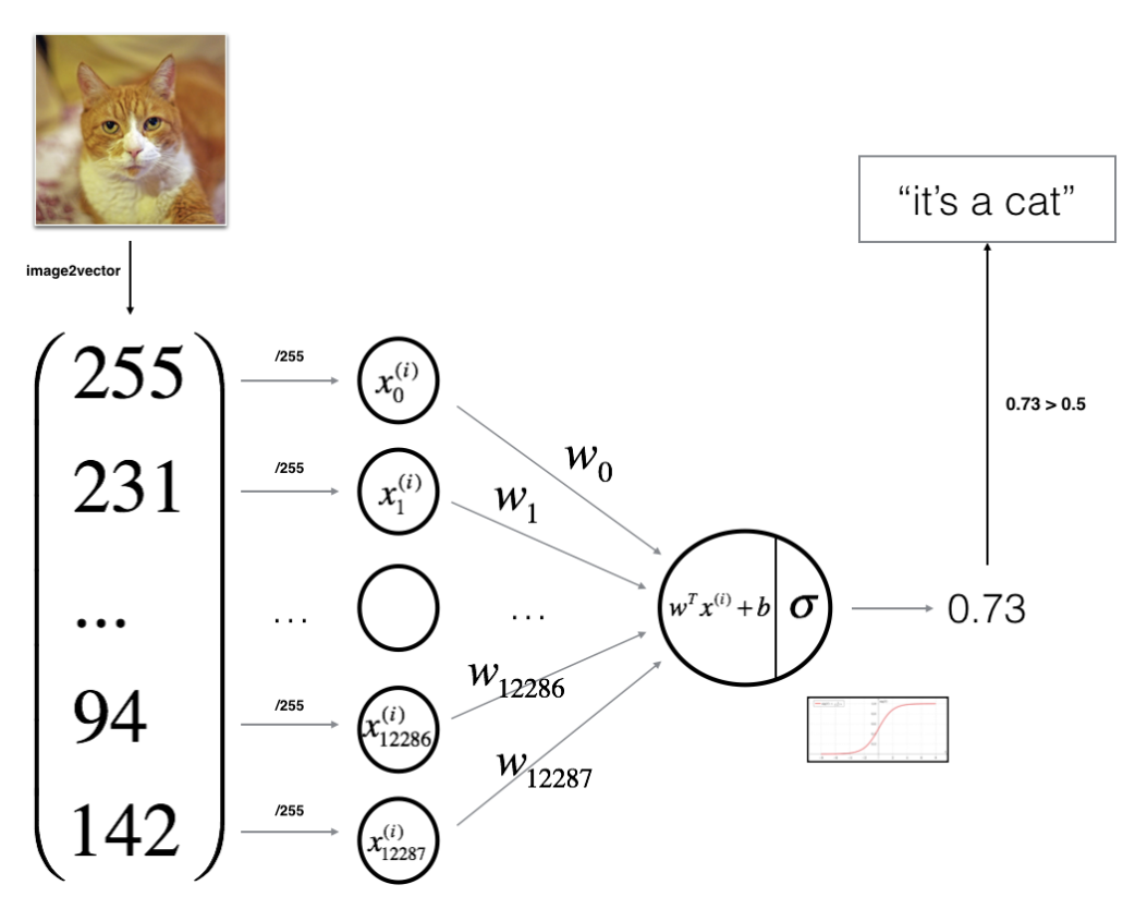
Neural Network

 

- 식으로 나타내면 다음과 같다.

    x(i)에 대하여:

        (1) z(i) = w^Tx(i) + b

        (2) ŷ(i) = a(i) = sigmoid(z(i))

        (3) L(a(i), y(i)) = -y(i)log(a(i)-(1-y(i))log(1-a(i)) 

 

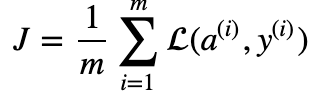
- cost function:

- Learning algorithm의 대략적인 steps:

    (1) 모델의 파라미터들을 초기화

    (2) cost 값을 최소화하는 파라미터 값들을 학습

    (3) 학습한 파라미터 값을 가지고 예측을 한다(on the test set)

    (4) 결과를 분석하고 평가

 

 

* Building the parts of our algorithm

 

- steps for building a NN:

    (1) 모델 구조를 정의한다(input의 갯수 등등)

    (2) 모델의 파라미터를 초기화한다.

    (3) Loop:

            - current loss 계산(forward propagation)

            - current gradient 계산(backward propagation)

            - parameters 업데이트(gradient descent)

 

1) Helper functions

 

- sigmoid function 사용

s = 1 / (1+np.exp(-z))

 

2) Initializing parameters

 

- np.zeros() function 사용하여 parameter들 ]을 초기화시킨다.

def initialize_with_zeros(dim):
    """
    This function creates a vector of zeros of shape (dim, 1) for w and initializes b to 0.
    
    Argument:
    dim -- size of the w vector we want (or number of parameters in this case)
    
    Returns:
    w -- initialized vector of shape (dim, 1)
    b -- initialized scalar (corresponds to the bias)
    """

    w = np.zeros((dim, 1))
    b = 0

    assert(w.shape == (dim, 1))
    assert(isinstance(b, float) or isinstance(b, int))
    
    return w, b
    
dim = 2
w, b = initialize_with_zeros(dim)
print ("w = " + str(w))
print ("b = " + str(b))

result: w = [[ 0.] [ 0.]] b = 0

 

- image input에 대해서는 w의 모양은 (height * width * channel, 1)

 

 

3) Forward and Backward propagation

 

- Forward Propagation:

    1) X

    2) A = sigmoid(w^T + b) = (a(1), a(2), a(3), ..., a(m-1), a(m))

    3) cost function:

- Backward Propagation:

   

 

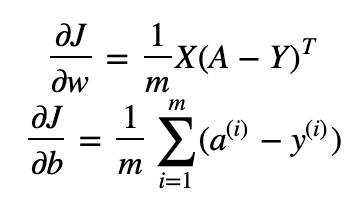
* np.dot(): 행렬 간 내적 곱 / np.log(): 로그 계산

 

 

def propagate(w, b, X, Y):
    """
    Implement the cost function and its gradient for the propagation explained above

    Arguments:
    w -- weights, a numpy array of size (num_px * num_px * 3, 1)
    b -- bias, a scalar
    X -- data of size (num_px * num_px * 3, number of examples)
    Y -- true "label" vector (containing 0 if non-cat, 1 if cat) of size (1, number of examples)

    Return:
    cost -- negative log-likelihood cost for logistic regression
    dw -- gradient of the loss with respect to w, thus same shape as w
    db -- gradient of the loss with respect to b, thus same shape as b
    
    Tips:
    - Write your code step by step for the propagation. np.log(), np.dot()
    """
    
    m = X.shape[1]
    
    # FORWARD PROPAGATION (FROM X TO COST)
    A = sigmoid(np.dot(w.T, X)+b) # compute activation
    cost = -(1/m)*(np.sum((Y*np.log(A))+((1-Y))*np.log(1-A))) # compute cost
    
    # BACKWARD PROPAGATION (TO FIND GRAD)
    dw = (1/m) * np.dot(X, (A-Y).T)
    db = (1/m) * np.sum(A-Y)

    assert(dw.shape == w.shape)
    assert(db.dtype == float)
    cost = np.squeeze(cost)
    assert(cost.shape == ())
    
    grads = {"dw": dw,
             "db": db}
    
    return grads, cost
    
w, b, X, Y = np.array([[1.],[2.]]), 2., np.array([[1.,2.,-1.],[3.,4.,-3.2]]), np.array([[1,0,1]])
grads, cost = propagate(w, b, X, Y)
print ("dw = " + str(grads["dw"]))
print ("db = " + str(grads["db"]))
print ("cost = " + str(cost))

result: dw = [[ 0.99845601] [ 2.39507239]] db = 0.00145557813678 cost = 5.80154531939

 

4) Optimization

 

- update parameters using gradient descent

- update rule: θ = θ - α*dθ 

 

def optimize(w, b, X, Y, num_iterations, learning_rate, print_cost = False):
    """
    This function optimizes w and b by running a gradient descent algorithm
    
    Arguments:
    w -- weights, a numpy array of size (num_px * num_px * 3, 1)
    b -- bias, a scalar
    X -- data of shape (num_px * num_px * 3, number of examples)
    Y -- true "label" vector (containing 0 if non-cat, 1 if cat), of shape (1, number of examples)
    num_iterations -- number of iterations of the optimization loop
    learning_rate -- learning rate of the gradient descent update rule
    print_cost -- True to print the loss every 100 steps
    
    Returns:
    params -- dictionary containing the weights w and bias b
    grads -- dictionary containing the gradients of the weights and bias with respect to the cost function
    costs -- list of all the costs computed during the optimization, this will be used to plot the learning curve.
    
    Tips:
    You basically need to write down two steps and iterate through them:
        1) Calculate the cost and the gradient for the current parameters. Use propagate().
        2) Update the parameters using gradient descent rule for w and b.
    """
    
    costs = []
    
    for i in range(num_iterations):
        
        
        # Cost and gradient calculation (≈ 1-4 lines of code)
        ### START CODE HERE ### 
        grads, cost = propagate(w, b, X, Y)
        ### END CODE HERE ###
        
        # Retrieve derivatives from grads
        dw = grads["dw"]
        db = grads["db"]
        
        # update rule (≈ 2 lines of code)
        ### START CODE HERE ###
        w = w - learning_rate * dw
        b = b - learning_rate * db
        ### END CODE HERE ###
        
        # Record the costs
        if i % 100 == 0:
            costs.append(cost)
        
        # Print the cost every 100 training iterations
        if print_cost and i % 100 == 0:
            print ("Cost after iteration %i: %f" %(i, cost))
    
    params = {"w": w,
              "b": b}
    
    grads = {"dw": dw,
             "db": db}
    
    return params, grads, costs
    
params, grads, costs = optimize(w, b, X, Y, num_iterations= 100, learning_rate = 0.009, print_cost = False)

print ("w = " + str(params["w"]))
print ("b = " + str(params["b"]))
print ("dw = " + str(grads["dw"]))
print ("db = " + str(grads["db"]))

result: w = [[ 0.19033591] [ 0.12259159]] b = 1.92535983008 dw = [[ 0.67752042] [ 1.41625495]] db = 0.219194504541

 

- update해 얻는 w, b를 가지고 label을 예측할 수 있다.

    (1) ŷ = A = sigmoid(w.T * X + b)

    (2) activation을 0/1(0.5 이상이면 1, 아니면 0)로 만들어준다.

 

def predict(w, b, X):
    '''
    Predict whether the label is 0 or 1 using learned logistic regression parameters (w, b)
    
    Arguments:
    w -- weights, a numpy array of size (num_px * num_px * 3, 1)
    b -- bias, a scalar
    X -- data of size (num_px * num_px * 3, number of examples)
    
    Returns:
    Y_prediction -- a numpy array (vector) containing all predictions (0/1) for the examples in X
    '''
    
    m = X.shape[1]
    Y_prediction = np.zeros((1,m))
    w = w.reshape(X.shape[0], 1)
    
    # Compute vector "A" predicting the probabilities of a cat being present in the picture
    A = sigmoid(np.dot(w.T, X) + b)
    
    for i in range(A.shape[1]):
        
        # Convert probabilities A[0,i] to actual predictions p[0,i]
        if A[0, i] >= 0.5:
            Y_prediction[0, i] = 1
        else:
            Y_prediction[0, i] = 0
    
    assert(Y_prediction.shape == (1, m))
    
    return Y_prediction
    
w = np.array([[0.1124579],[0.23106775]])
b = -0.3
X = np.array([[1.,-1.1,-3.2],[1.2,2.,0.1]])
print ("predictions = " + str(predict(w, b, X)))

result: predictions = [[ 1. 1. 0.]]

 

 

 

* Merge all functions into a model

 

def model(X_train, Y_train, X_test, Y_test, num_iterations = 2000, learning_rate = 0.5, print_cost = False):
    """
    Builds the logistic regression model by calling the function you've implemented previously
    
    Arguments:
    X_train -- training set represented by a numpy array of shape (num_px * num_px * 3, m_train)
    Y_train -- training labels represented by a numpy array (vector) of shape (1, m_train)
    X_test -- test set represented by a numpy array of shape (num_px * num_px * 3, m_test)
    Y_test -- test labels represented by a numpy array (vector) of shape (1, m_test)
    num_iterations -- hyperparameter representing the number of iterations to optimize the parameters
    learning_rate -- hyperparameter representing the learning rate used in the update rule of optimize()
    print_cost -- Set to true to print the cost every 100 iterations
    
    Returns:
    d -- dictionary containing information about the model.
    """
    
    
    # initialize parameters with zeros (≈ 1 line of code)
    w, b = initialize_with_zeros(X_train.shape[0])

    # Gradient descent (≈ 1 line of code)
    parameters, grads, costs = optimize(w, b, X_train, Y_train, num_iterations, learning_rate, print_cost = False)
    
    # Retrieve parameters w and b from dictionary "parameters"
    w = parameters["w"]
    b = parameters["b"]
    
    # Predict test/train set examples (≈ 2 lines of code)
    Y_prediction_test = predict(w, b, X_test)
    Y_prediction_train = predict(w, b, X_train)


    # Print train/test Errors
    print("train accuracy: {} %".format(100 - np.mean(np.abs(Y_prediction_train - Y_train)) * 100))
    print("test accuracy: {} %".format(100 - np.mean(np.abs(Y_prediction_test - Y_test)) * 100))

    
    d = {"costs": costs,
         "Y_prediction_test": Y_prediction_test, 
         "Y_prediction_train" : Y_prediction_train, 
         "w" : w, 
         "b" : b,
         "learning_rate" : learning_rate,
         "num_iterations": num_iterations}
    
    return d
    
d = model(train_set_x, train_set_y, test_set_x, test_set_y, num_iterations = 2000, learning_rate = 0.005, print_cost = True)

result: train accuracy: 99.04306220095694 % test accuracy: 70.0 %

 

* Further analysis_Choices of learning rate

 

- learning rate는 얼마나 빠르게 parameter들을 update 시킬지를 결정한다.

- learning rate가 너무 크면 optimal value를 overshoot하게 되며, 너무 작으면 best한 값을 찾기 위해 수렴하기까지 많은 iteration 과정이 필요하다. 

 

result:

learning rate is: 0.01

train accuracy: 99.52153110047847 %

test accuracy: 68.0 %

-------------------------------------------------------

learning rate is: 0.001

train accuracy: 88.99521531100478 %

test accuracy: 64.0 %

-------------------------------------------------------

learning rate is: 0.0001

train accuracy: 68.42105263157895 %

test accuracy: 36.0 %

 

- learning rate가 너무 크면 cost가 너무 많이 진동하게 되면서 그래프를 벗어나게 될 수도 있다.(예시에서는 잘 나왔을 뿐)

- 너무 작으면 overfitting이 발생할 가능성이 높다,

- 따라서 cost function을 잘 최소화 시킬 수 있는 learning rate을 선택해야 하며 overfitting이 발생할 경우에는 이를 줄일 수 있는 technique들을 사용해야 한다.

 

---

1. 데이터셋의 전처리가 중요하다.

2. 세부 과정들을 separate하게 만든 다음, 나중에 하나의 함수로 합친다.(initialize(), propagate(), optimize() -> model())

3. learning rate를 tuning하는 것이 알고리즘에 큰 차이를 낳을 수 있다.